
Regularization - Overfitting in the Real World (and How to Fight It)
Overfitting is what happens when your model memorizes training data. Regularization is the practical tool that keeps it honest.
Axel Domingues
If I had to summarize the biggest trap in early Machine Learning learning, it’s this:
A model can look amazing on paper and still fail the moment it meets real data.
That’s overfitting.
Spot it fast
Training looks great, but validation/test drops hard. Boundaries look “too wiggly”. Small input changes cause big output changes.
Why it happens
Too many features for the data, feature mapping/polynomials, noisy labels, or simply not enough examples.
Fix it in practice
Regularization (lambda), reduce feature mapping degree, add more data, and choose hyperparameters using a validation set.
And it’s not just a theoretical problem — it’s a production problem:
- it wastes time (you keep tweaking the wrong thing)
- it wastes money (you ship a model that fails silently)
- it kills trust (stakeholders stop believing your metrics)
Regularization shows up early in the course (notably in logistic regression with feature mapping) because it’s the first time you can build a model that is powerful enough to fool you.
What overfitting looks like (in plain words)
Overfitting is when the model:
- learns the training set extremely well
- but fails on new examples
In practice, you’ll see things like:
- very high training accuracy
- poor validation/test accuracy
- decision boundaries that look “too wiggly”
- predictions that are unstable for small changes in input
If your model performance drops a lot when you move from training to validation, don’t assume “we need a better algorithm.” Assume overfitting until proven otherwise.
Why overfitting happens
In the course (and in real projects), overfitting tends to come from one of these:
The model has enough knobs to match the training set perfectly — even when the pattern is partly noise.
Mapping 2 inputs into many polynomial features makes the boundary extremely flexible (and easy to overfit).
With limited data, the model can’t learn a stable signal, so it learns quirks.
If labels contain errors or randomness, the model can “learn the noise” instead of the underlying rule.
The most common “Course moment” where overfitting becomes obvious is when you map 2 input features into many polynomial features (like the microchip dataset in Exercise 2).
At that point, the model is capable of drawing a very complex boundary — complex enough to perfectly match the training data.
And that’s the problem.
Regularization: the idea
Regularization is a rule you add to training:
Prefer simpler parameter values unless the data strongly justifies complexity.
In the course, the main regularization used is L2 regularization (penalize large weights).
In plain terms:
- you still want low prediction error
- but you also want parameters (
theta) that don’t explode
So training becomes “error + penalty.”
Base loss: fit the data
You still want predictions to match the training examples.
Penalty: discourage extreme weights
You add a cost for large parameter values so the model can’t get overly “wiggly” unless the data demands it.
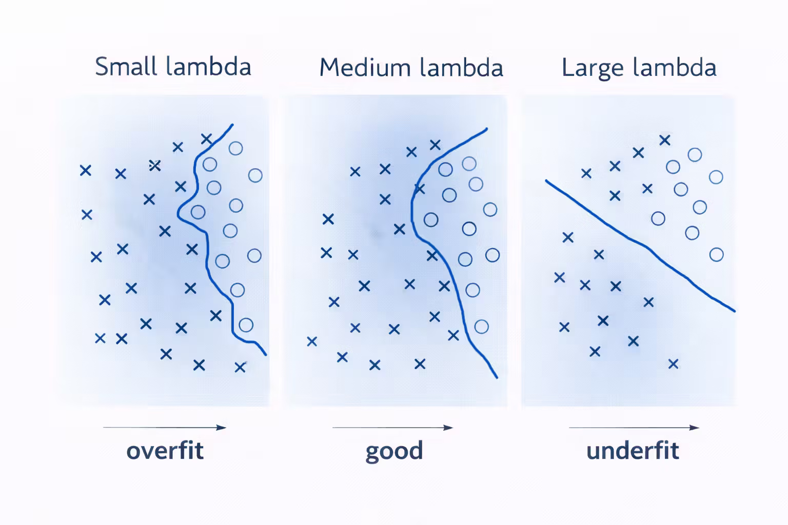
Lambda controls the tradeoff
Small lambda → more freedom (higher overfitting risk)
Large lambda → less freedom (higher underfitting risk)
The strength of that penalty is controlled by lambda (lambda).
The lambda knob (how it changes model behavior)
Lambda is one of the first real “hyperparameters” that feels like a control knob.
- weak penalty
- weights can grow large
- boundary can become complex
- higher risk of overfitting
- weights stay under control
- boundary becomes smoother
- usually better generalization
- strong penalty
- weights shrink toward zero
- boundary becomes too simple
- can underfit
The “best” lambda is not a constant. It depends on your dataset size, feature mapping, noise level, and how you measure success.
Implementation detail that matters: don’t regularize the intercept
In the course implementations, the intercept term is treated specially.
In Octave indexing:
theta(1)is the intercept parameter
You typically do not regularize it.
theta(1) by mistake, your decision boundary can shift in confusing ways and you’ll waste time blaming the optimizer.A common pattern is:
theta_reg = theta;
theta_reg(1) = 0;
Then use theta_reg only in the penalty terms.
Why? Because the intercept is a baseline shift. Penalizing it can shift the whole boundary in ways that don’t match the intended behavior.
This is an easy bug to make: everything runs, your boundary looks “off,” and you waste time blaming the optimizer.
Regularized logistic regression (the Exercise 2 pattern)
This is the “classic” regularized logistic regression implementation style used in the course.
function [J, grad] = costFunctionReg(theta, X, y, lambda)
  m = length(y);

  h = sigmoid(X * theta);

  theta_reg = theta;
  theta_reg(1) = 0;

  J = (1/m) * sum( -y .* log(h) - (1 - y) .* log(1 - h) ) ...
      + (lambda/(2*m)) * sum(theta_reg .^ 2);

  grad = (1/m) * (X' * (h - y)) + (lambda/m) * theta_reg;
end
Even if you don’t memorize the expression, remember the structure:
- compute predictions
h - compute base loss
- add weight penalty (skip intercept)
- compute base gradient
- add penalty gradient (skip intercept)
Regularized linear regression (same concept)
Regularization isn’t specific to logistic regression.
If you were to regularize linear regression in the same style, the pattern is identical:
- keep the intercept unpenalized
- add penalty to cost and gradient
The math changes, the habit does not.
How to pick lambda (the engineer workflow)
It’s tempting to pick a lambda once and move on.
But the right way (even for small projects) is:
- try a small set of lambda values
- evaluate on a validation set
- pick the best one based on the metric you care about
A practical grid
lambda in {0, 0.01, 0.1, 1, 10}
Then:
- train model for each lambda
- compute validation accuracy (or validation cost)
- choose the lambda that performs best on validation
Don’t pick lambda using the test set. The test set is your final exam.
The three-split habit (training / validation / test)
This is the workflow I started adopting from the course and kept:
- Training set: fit parameters (learn theta)
- Validation set: choose hyperparameters (like lambda)
- Test set: final unbiased evaluation
If you don’t do this, you can accidentally “overfit your decisions” even when the model seems regularized.
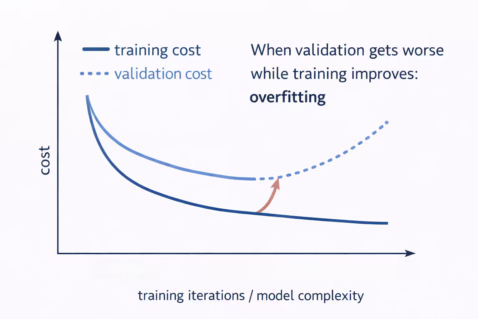
How to recognize overfitting fast
Here are quick signals that saved me time:
- training accuracy is much higher than validation accuracy
- validation cost starts increasing while training cost keeps decreasing
- decision boundary looks unnecessarily complex
- small data changes cause big parameter changes
If I see these, I immediately try:
- increasing lambda
- reducing feature mapping degree
- adding more data
Debugging checklist for regularization code
When regularization breaks, it tends to break in predictable ways:
Most likely you regularized the intercept (theta(1)).
Fix: set theta_reg(1) = 0 before applying penalty terms.
Lambda term missing from cost (or missing /m scaling).
Quick sanity: same theta + higher lambda should not make cost smaller.
Regularization term missing from gradient, or element-wise ops are wrong (.^, .*).
Check shapes: size(X), size(theta), size(y).
Lambda might be too large, or feature mapping degree is too low for the pattern.
Quick checks:
size(X)
size(theta)
size(y)
And print costs for a couple of lambda values to verify the cost increases as lambda increases.
A nice sanity check: with the same theta, increasing lambda should never make the cost smaller (because you’re adding a penalty).
What I’m keeping from this lesson
- Overfitting is the default risk once a model becomes expressive.
- Regularization is a practical constraint that improves generalization.
- Lambda is a tool, not a magic number.
- Validation-driven selection is the correct way to choose lambda.
- The intercept term should not be regularized (in the course conventions).
What’s Next
Next up is where the course starts feeling like “real ML”: handwritten digits.
I’ll build a multi-class digit classifier using one-vs-all logistic regression, then run a small neural network forward pass on the same dataset to see how a pre-trained network makes predictions.
Exercise 3 - One-vs-All + Intro to Neural Networks (Handwritten Digits!)
Build a multi-class digit classifier with one-vs-all logistic regression, then run a small neural network forward pass on the same dataset.
Exercise 2 - Logistic Regression for Classification (My First Real Classifier)
My first real classifier - predict admissions from exam scores with logistic regression, then learn why regularization matters on a non-linear dataset.