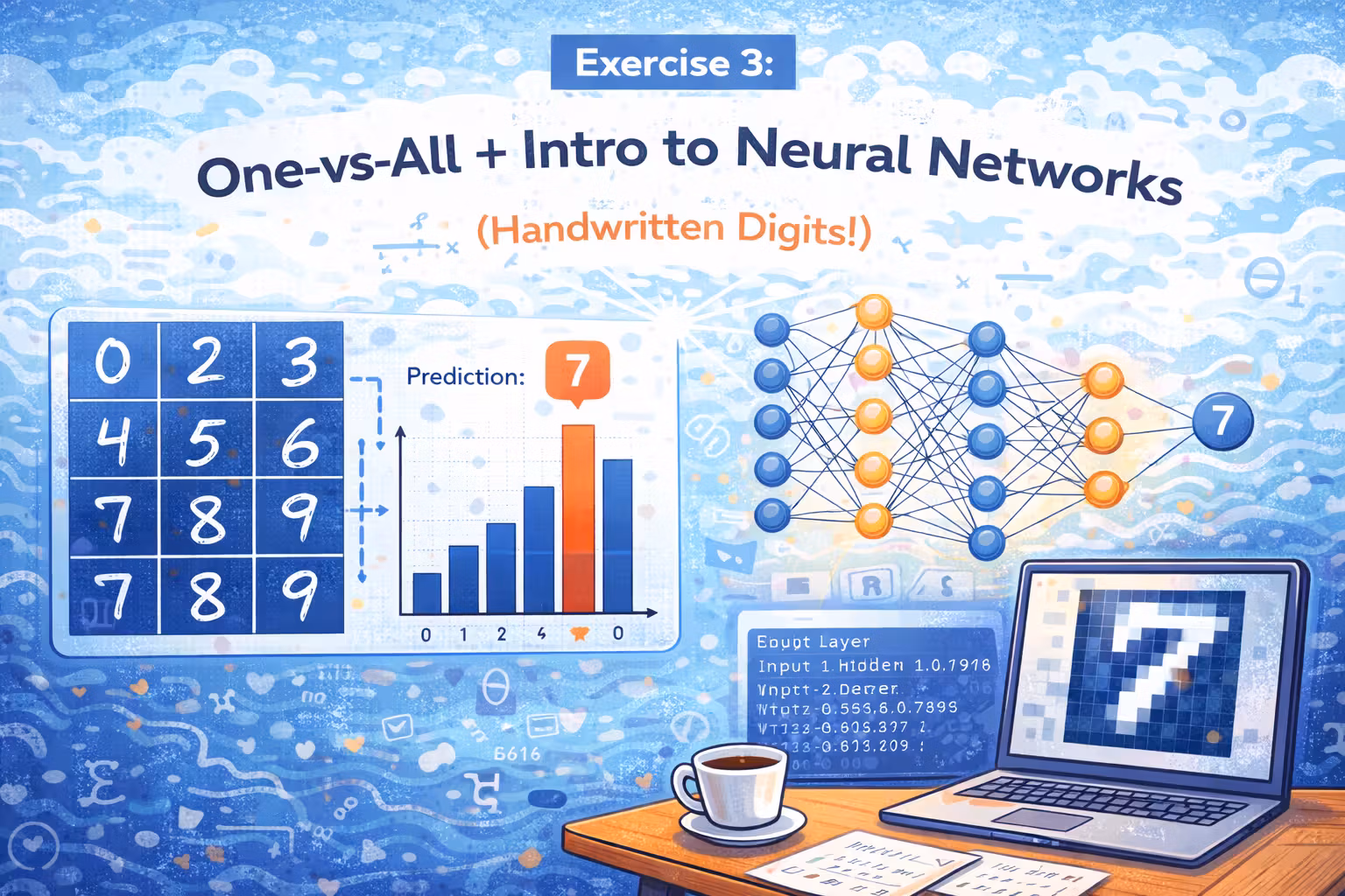
Exercise 3 - One-vs-All + Intro to Neural Networks (Handwritten Digits!)

Exercise 3 is where ML stopped being “toy problems” for me.

We’re classifying handwritten digits (0–9) from pixel data — the kind of task you can actually imagine in a product:

• reading postal codes
• recognizing amounts on checks
• parsing handwritten forms

The assignment has two parts:

1. One-vs-all logistic regression (multi-class classification)
2. A neural network forward pass (same dataset, pre-trained weights)

What’s inside the Exercise 3 bundle

The scripts (ex3.m, ex3_nn.m) are designed like a guided debugger: run them top-to-bottom and validate each checkpoint before moving on.

Dataset: 5000 digits, 20x20 pixels, flattened into 400 features

The dataset has:

• 5000 training examples
• each example is a 20 by 20 grayscale image
• each image is “unrolled” into a 400-dimensional row vector

So X is a 5000 by 400 matrix.

There’s one detail that will bite you if you don’t read it:

• the digit 0 is mapped to the label 10 (because Octave indexing starts at 1)

If your model seems to never predict 0, check your label mapping. In this dataset, “0” is label 10.

Step 0 — Visualize the data (because it’s motivating)

The first thing the script does is show a grid of random digits using displayData.m.

This is not optional for me.

When you’re debugging a model, being able to see the input makes it easier to sanity-check:

• are the pixels shaped correctly?
• are the digits readable?
• did I accidentally transpose or reorder features?

If the digits look like noise, don’t even start training.

Part 1 — One-vs-all logistic regression

The idea

Logistic regression is naturally a binary classifier.

One-vs-all turns it into a multi-class classifier by training K separate binary classifiers, one per class:

• classifier 1: “is it a 1?”
• classifier 2: “is it a 2?”
• …
• classifier 10: “is it a 0?” (remember: 0 maps to 10)

At prediction time:

• run all K classifiers
• pick the class with the highest predicted probability

Implement lrCostFunction.m (regularized logistic regression)

This is the heart of Part 1.

lrCostFunction computes:

• cost J
• gradient grad

And it includes regularization.

Key implementation rule:

• do not regularize the intercept term (theta(1))

Vectorized implementation pattern:

function [J, grad] = lrCostFunction(theta, X, y, lambda)
  m = length(y);

  h = sigmoid(X * theta);

  theta_reg = theta;
  theta_reg(1) = 0;

  J = (1/m) * sum( -y .* log(h) - (1 - y) .* log(1 - h) ) ...
      + (lambda/(2*m)) * sum(theta_reg .^ 2);

  grad = (1/m) * (X' * (h - y)) + (lambda/m) * theta_reg;
end

If fmincg behaves strangely later, it’s usually because your gradient is wrong or you accidentally regularized theta(1).

Train all classifiers in oneVsAll.m

Now we train K classifiers.

Practical flow:

• add intercept column to X
• loop over classes c = 1..K
• create a binary label vector: y_c = (y == c)
• optimize theta for that class
• store each theta row in all_theta

A typical structure:

all_theta = zeros(num_labels, n + 1);

for c = 1:num_labels
  initial_theta = zeros(n + 1, 1);
  y_c = (y == c);

  options = optimset('MaxIter', 50);

  [theta] = fmincg(@(t)(lrCostFunction(t, X, y_c, lambda)), initial_theta, options);

  all_theta(c, :) = theta';
end

Two important engineering observations here:

• looping over classes is fine (K is small)
• inside each class optimization, everything should be vectorized

Predict with predictOneVsAll.m (vectorization payoff)

This is where the matrix mindset becomes worth it.

Instead of predicting digit-by-digit in a loop, we predict for all examples and all classes in one shot.

Typical approach:

• compute probabilities for every class
• take the argmax per example

probs = sigmoid(X * all_theta');
[~, p] = max(probs, [], 2);

p is your predicted label.

Checkpoint from the assignment:

• training accuracy is about 94.9% for one-vs-all logistic regression

This accuracy is on the training set (not a true generalization measure), but it’s a great “did I implement it correctly?” checkpoint.

Part 2 — Neural Networks (forward propagation only)

After one-vs-all, the assignment introduces a small neural network.

Important: in Exercise 3, you do not train the neural network.

You’re given pre-trained weights (Theta1 and Theta2) and you implement prediction via forward propagation.

This is basically: “use a neural network as a function.”

Understanding the network shape

The network has:

• input layer: 400 pixel features (+ intercept)
• one hidden layer (25 units is typical in this exercise)
• output layer: 10 units (digits 1–10, where 10 represents digit 0)

The weights are stored as matrices:

• Theta1 maps input layer to hidden layer
• Theta2 maps hidden layer to output layer

Most bugs here are shape/indexing bugs. Print sizes early and often.

Implement predict.m (neural network)

The forward pass is a sequence of matrix multiplies + sigmoid activations.

Implementation pattern:

function p = predict(Theta1, Theta2, X)
  m = size(X, 1);

  a1 = [ones(m, 1) X];

  z2 = a1 * Theta1';
  a2 = sigmoid(z2);
  a2 = [ones(m, 1) a2];

  z3 = a2 * Theta2';
  a3 = sigmoid(z3);

  [~, p] = max(a3, [], 2);
end

Checkpoint from the assignment:

• accuracy is about 97.5% using the provided neural network weights

After that, ex3_nn.m typically shows an interactive sequence:

• display a digit
• print the predicted label
• move to the next example until you stop it

That interactive viewer was one of the most motivating things in the early course.

Why vectorization mattered (for real this time)

At this point, the dataset is big enough that slow code becomes painful:

• 5000 examples
• 400 features
• 10 classifiers

If you try to compute gradients with nested loops over examples and features, Octave will punish you.

Vectorization gave me two wins:

• speed: training completes in reasonable time
• correctness: matrix operations reduce index mistakes

Vectorization isn’t just a performance trick. It’s how you keep the implementation aligned with the model you think you’re building.

Debugging checklist (things I actually used)

When Exercise 3 breaks, it usually breaks in predictable ways:

• forgot to add the intercept column to X
• regularized theta(1) by mistake
• mixed up dimensions for Theta1 / Theta2 (forgot transpose)
• label “0” mapped to 10 (and you didn’t account for it)
• using matrix ops where element-wise ops were intended

My first-line debugging tools:

size(X)
size(theta)
size(all_theta)
size(Theta1)
size(Theta2)

And I always re-run the scripts from the top.

What I’m keeping from Exercise 3

• One-vs-all is a clean engineering pattern for multi-class classification.
• Regularization is essential once you have lots of parameters.
• Forward propagation is just “stacked feature transforms” + sigmoid.
• Pretrained weights are a great way to learn prediction before learning training.
• Vectorization turns ML code from fragile to robust.

What’s Next

Next up is the big leap: training a neural network.

I’ll implement backpropagation for a 2-layer network, verify gradients with numerical gradient checking, then train on handwritten digits and push toward ~95% accuracy with my own learned weights (not pre-trained ones).