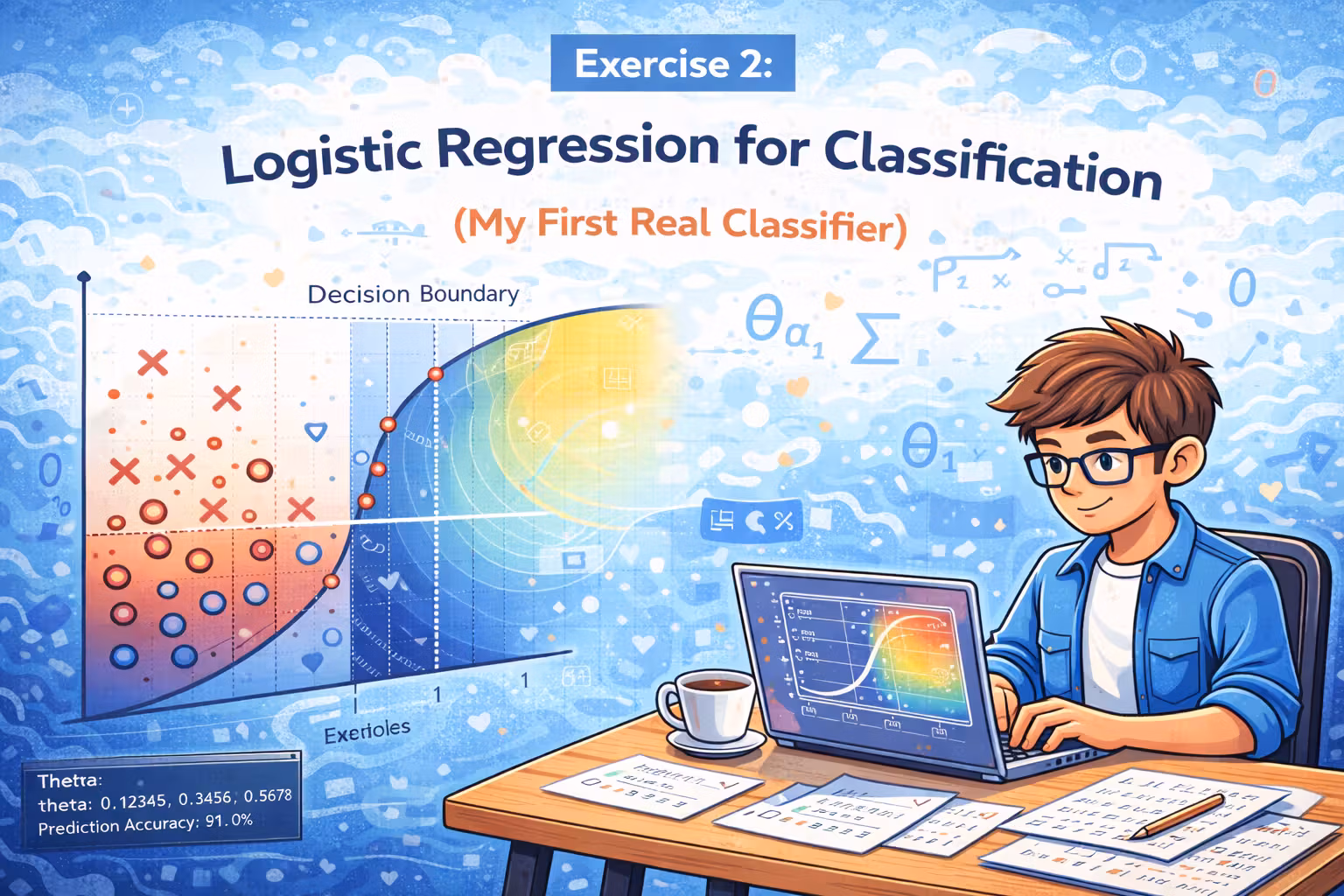
Exercise 2 - Logistic Regression for Classification (My First Real Classifier)

Exercise 1 taught me how to predict a number.

Exercise 2 is where things start to feel like “real ML”: classification.

Instead of predicting profit or price, we predict a label:

• 1 = yes (admit / accept)
• 0 = no (reject)

This exercise is split into two parts:

1. Logistic regression on an admissions dataset (mostly linear boundary)
2. Regularized logistic regression on a microchip QA dataset (non-linear boundary)

What’s inside the Exercise 2 bundle

Part 1 — University admissions (my first classifier)

Step 1 — Plot the data (always)

The admissions dataset contains two exam scores per student and a label (admitted / not admitted).

Plotting answers the first honest question: does a straight boundary look plausible?

If you’re using a helper like plotData.m, the pattern is usually:

• one marker for admitted
• another marker for not admitted

This plot becomes the background for the decision boundary later.

If your plot looks strange (all points stacked, weird scales), stop. Don’t debug ML with broken data visualization.

Sigmoid: turning scores into probabilities

Logistic regression works by producing a probability between 0 and 1.

The sigmoid function is the basic building block:

function g = sigmoid(z)
  g = 1 ./ (1 + exp(-z));
end

Two things I learned immediately:

• you want this to work for scalars AND vectors/matrices
• you want it vectorized so you can compute probabilities for all examples in one line

Cost + gradient: the contract between your model and the optimizer

The key implementation in Part 1 is costFunction.m. It should return:

• J: a single number (how wrong you are)
• grad: a vector (direction to improve theta)

A clean vectorized pattern:

function [J, grad] = costFunction(theta, X, y)
  m = length(y);

  h = sigmoid(X * theta);

  J = (1/m) * sum( -y .* log(h) - (1 - y) .* log(1 - h) );

  grad = (1/m) * (X' * (h - y));
end

Checkpoint: cost at zero theta

When theta starts at zeros, the cost should be around 0.693.

This number is incredibly useful.

If your cost is not close to 0.693 at zero theta, do not continue. Fix costFunction.m first.

Optimize theta with fminunc (no manual gradient descent)

In Exercise 2, the course introduces a practical workflow:

• you implement cost + gradient correctly
• you let a solver (fminunc) handle the optimization steps

The call pattern looks like:

options = optimset('GradObj', 'on', 'MaxIter', 400);
[theta, cost] = fminunc(@(t)(costFunction(t, X, y)), initial_theta, options);

What I liked about this approach:

• no learning rate tuning
• faster iterations while learning
• forces correctness of gradient (because the solver relies on it)

If fminunc behaves strangely, it’s usually a bug in your gradient or shape mismatch in X, theta, or y.

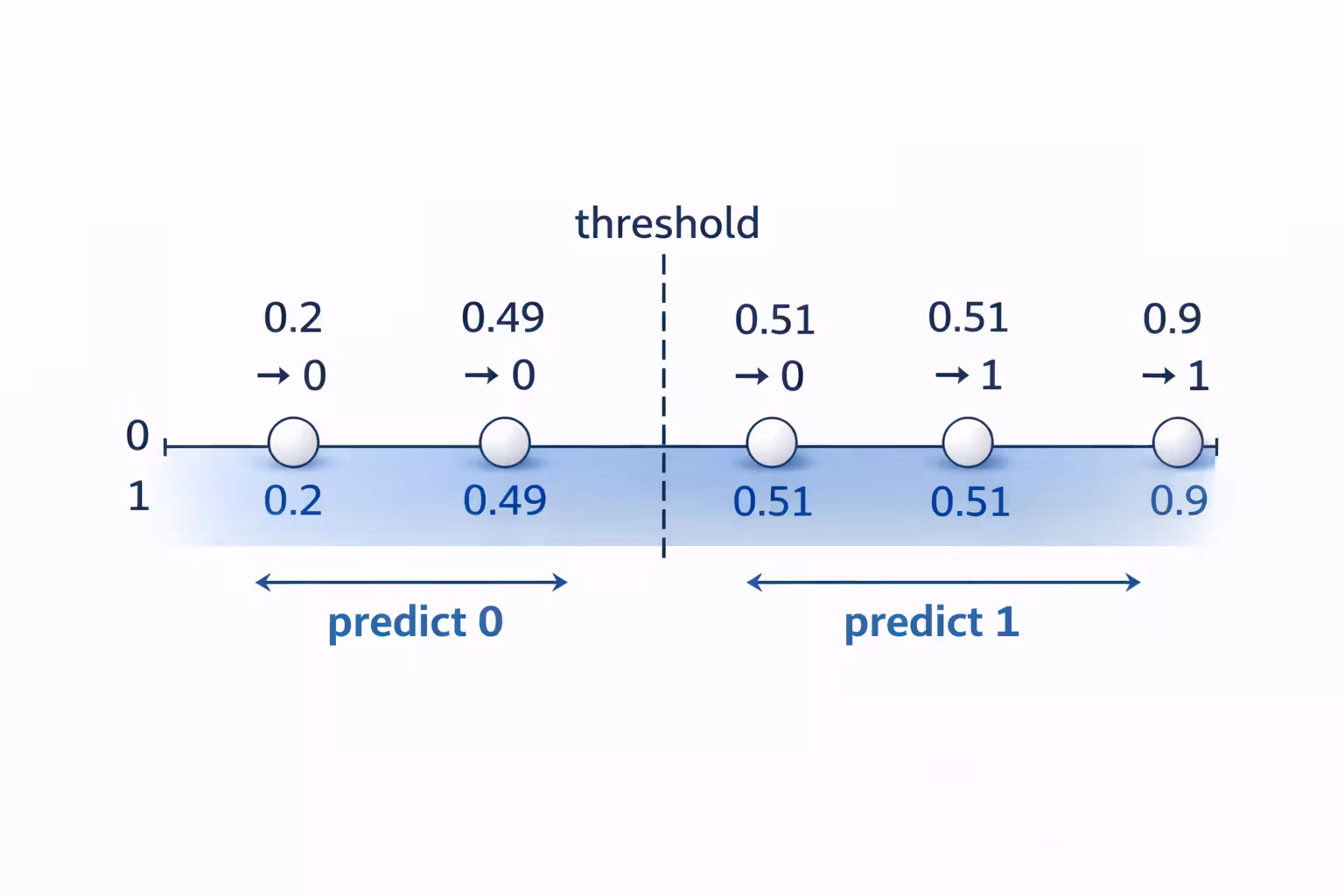
Predict: turn probabilities into decisions

Once you have theta, you can predict:

• probability = sigmoid(X * theta)
• prediction = probability >= 0.5

A simple predict.m:

function p = predict(theta, X)
  p = sigmoid(X * theta) >= 0.5;
end

Then compute training accuracy:

• compare p with y
• compute percent correct

This is the first moment where it felt like a real classifier: it makes decisions from data.

Part 2 — Microchip QA (non-linear boundary + regularization)

The second dataset has two test results for microchips and a label:

• accepted = 1
• rejected = 0

The twist: a straight line can’t separate the classes well.

So the course does two things:

1. Feature mapping (make the model more expressive)
2. Regularization (prevent overfitting)

Feature mapping: make a non-linear boundary possible

mapFeature.m is provided and expands the two input features into a set of polynomial features.

This changes the shape of the data the model sees:

• before mapping: 2 features (+ intercept)
• after mapping: many more features

This is powerful… and dangerous.

More features means a more flexible boundary, which means the model can start “memorizing” the training set.

Regularization: controlling complexity with lambda

You implement costFunctionReg.m which adds a penalty for large parameter values.

Important rule from the course:

• do not regularize the intercept term (theta(1) in Octave)

Implementation pattern:

function [J, grad] = costFunctionReg(theta, X, y, lambda)
  m = length(y);

  h = sigmoid(X * theta);

  theta_reg = theta;
  theta_reg(1) = 0; % do not penalize intercept

  J = (1/m) * sum( -y .* log(h) - (1 - y) .* log(1 - h) ) ...
      + (lambda/(2*m)) * sum(theta_reg .^ 2);

  grad = (1/m) * (X' * (h - y)) + (lambda/m) * theta_reg;
end

The lambda knob (intuition)

When you play with lambda, you get three regimes:

• small lambda: boundary becomes very complex, often overfits
• medium lambda: boundary simplifies and generalizes better
• large lambda: boundary becomes too simple, underfits

This is the first exercise where “overfitting” becomes visible.

If you only remember one thing from this section: feature mapping increases power, regularization keeps it honest.

Debugging checklist (what saved me time)

When this exercise breaks, it usually breaks in predictable ways:

• Shapes are wrong
  • check size(X), size(theta), size(y)
• Element-wise operators are missing
  • use .* and ./ where appropriate
• Log is blowing up
  • if h becomes 0 or 1 exactly, log(h) can be problematic
  • this usually points to numerical issues or unstable parameters
• Intercept is incorrectly regularized
  • remember to set theta_reg(1) = 0

The most dangerous bug is a wrong gradient: the script runs, the solver returns a theta, and your boundary looks “kind of random.” Use checkpoints and plot the boundary.

What I’m keeping from Exercise 2

• A classifier is a probability model + a decision threshold.
• Sigmoid must be vectorized.
• Cost + gradient is the core interface.
• Using an optimizer (fminunc) is a practical pattern.
• Feature mapping makes non-linear boundaries possible.
• Regularization (lambda) is what prevents “perfect training accuracy” from becoming a trap.

What’s Next

Next up is a topic that shows up everywhere once you see it: overfitting.

Overfitting is what happens when your model memorizes training data.
Regularization is the practical tool that keeps it honest — letting you keep model power without turning “perfect training accuracy” into a trap.