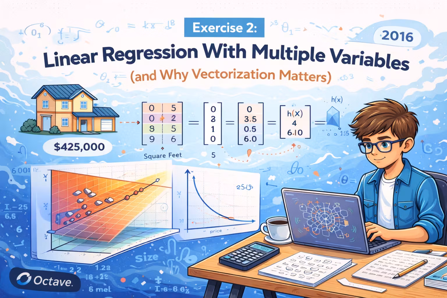
Linear Regression With Multiple Variables (and Why Vectorization Matters)

After Exercise 1, linear regression feels almost too easy: one feature, one line, gradient descent converges.

Then the course does the most realistic thing possible:

It adds more features.

In the real world you rarely have “profit depends on one number.” You have multiple inputs (size, number of rooms, location signals, time effects, etc.). This part of the course is where I learned two practical lessons that keep showing up in every ML system I’ve touched since:

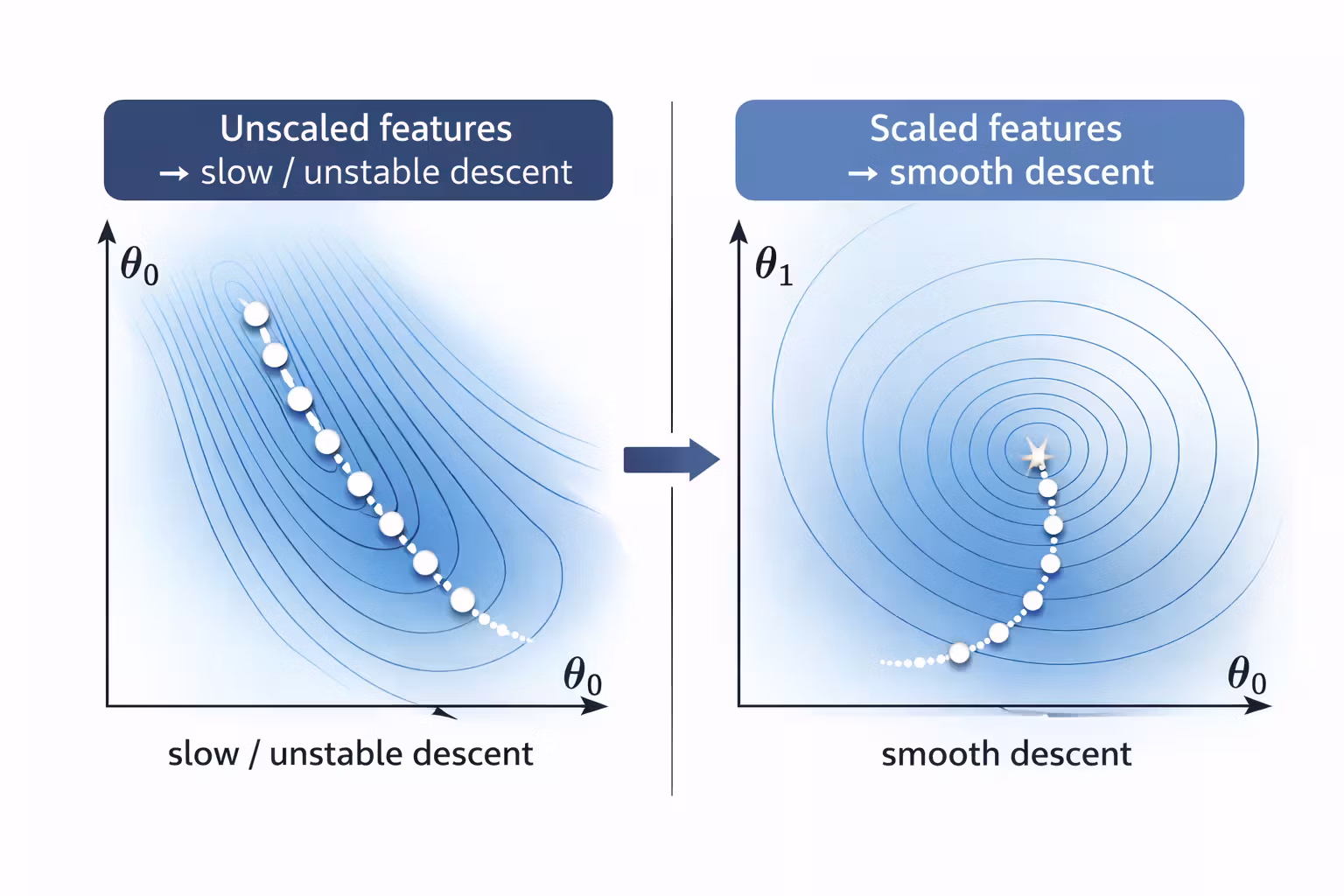
1. Feature scaling is not optional if you want gradient descent to converge.
2. Vectorization is not an optimization — it’s the cleanest way to keep the math and the code aligned.

What changes when you go from 1 feature to many

Single-variable linear regression is basically: “learn a line.”

Multi-variable linear regression is: “learn a weighted sum of features.”

In code terms:

• X becomes an m x (n+1) matrix (m examples, n features + intercept column)
• theta becomes a (n+1) x 1 vector
• predictions are still just:

predictions = X * theta;

Same idea, bigger surface area for bugs.

Files involved (typical course structure)

Walkthrough (do this in order)

Inspect feature scales (the “why is this not learning?” moment)

If one feature ranges in the thousands and another ranges 1–5, gradient descent may crawl or diverge.
Scaling isn’t optional — it’s what makes the optimization problem well-behaved.

Feature normalization (mean normalization + scaling)

The course’s approach is straightforward:

• subtract the mean for each feature
• divide by a scale (often standard deviation)

In Octave this usually looks like:

function [X_norm, mu, sigma] = featureNormalize(X)
  mu = mean(X);
  X = X - mu;
  sigma = std(X);
  X_norm = X ./ sigma;
end

Two notes I wrote down:

• Save mu and sigma because you need them to normalize new inputs later.
• Be careful with element-wise operations (./) vs matrix operations.

If you normalize training data but forget to normalize your prediction input, your predictions will be nonsense.

Update the design matrix

Once features are normalized, you still build X the same way:

• intercept column of ones
• normalized features

X = [ones(m, 1), X_norm];
theta = zeros(n + 1, 1);

This consistency is what makes the course great: the model doesn’t change — just the number of columns.

Cost function (multi-variable version)

The multi-variable cost computation is the same logic as Exercise 1:

• predict
• compute errors
• square and average

Vectorized implementation:

function J = computeCostMulti(X, y, theta)
  m = length(y);
  errors = (X * theta) - y;
  J = (1/(2*m)) * (errors' * errors);
end

The cost function is your contract. If cost behaves weirdly, fix cost first.

Gradient descent (multi-variable version)

The update is still the same pattern. The big improvement is that the vectorized gradient scales naturally with the number of features.

function [theta, J_history] = gradientDescentMulti(X, y, theta, alpha, num_iters)
  m = length(y);
  J_history = zeros(num_iters, 1);

  for iter = 1:num_iters
    errors = (X * theta) - y;
    theta = theta - (alpha/m) * (X' * errors);
    J_history(iter) = computeCostMulti(X, y, theta);
  end
end

If you compare this to a version with explicit loops over:

• iterations
• parameters
• training examples

…you immediately see why vectorization matters.

Why vectorization matters (beyond speed)

I initially thought vectorization was just about performance.

It’s not. It’s about correctness and clarity.

1) Vectorization reduces bug surface

When you write loops, you introduce:

• indexing mistakes
• off-by-one errors
• wrong accumulation
• forgetting to update parameters simultaneously

The vectorized form makes the update look like a single coherent operation.

2) Vectorization keeps the code aligned with the math

Even if you never show the formulas, the idea is:

• X * theta means “predict all examples”
• X' * errors means “aggregate how each feature contributed to the error”

That mapping makes it easier to reason about what’s happening.

3) Vectorization forces you to think in shapes

My most useful debugging tool in Octave became:

size(X)
size(theta)
size(y)

If shapes match expectations, everything downstream tends to behave.

The worst ML bugs are silent: the code runs and produces numbers, but they’re wrong. Shape checks catch a surprising amount of that.

Choosing alpha (learning rate) in practice

With multiple variables, alpha sensitivity becomes obvious.

What I did:

• start small (example: 0.01)
• plot or print cost every N iterations
• if cost decreases smoothly, try a slightly larger alpha
• if cost explodes (Inf / NaN), alpha is too large

A simple diagnostic snippet:

if mod(iter, 50) == 0
  fprintf('Iter %d | Cost: %f\n', iter, J_history(iter));
end

Treat cost history like logs. If your system has no telemetry, you’re guessing.

Optional: Normal Equation (when you don’t want iterations)

The course introduces an alternative approach: compute theta in one shot (no gradient descent).

In Octave, the canonical implementation is:

theta = pinv(X' * X) * X' * y;

When I first saw this, I loved it — it feels like cheating.

But the tradeoff is practical:

• it can be slower or less practical as feature count grows
• it relies on matrix operations that can be expensive

For learning purposes, it’s a great comparison tool:

• if normal equation and gradient descent give similar theta, your implementation is probably correct.

“Engineering notes” I’d keep even outside coursework

• Always normalize features when using gradient descent.
• Save normalization parameters (mu, sigma) for inference time.
• Prefer vectorized implementations — they’re easier to verify.
• Monitor training with cost history.
• Use normal equation as a correctness cross-check (when feasible).

What’s Next

Next up is a key comparison that upgrades your intuition fast: two ways to fit linear regression.

Same goal — find good parameters — different tradeoffs:

• Gradient descent: iterative improvements, great when you want training telemetry and you’re comfortable tuning alpha.
• Normal equation: one-shot solution, great for small problems and as a correctness cross-check.

Once you see both side by side, linear regression stops being “a model” and becomes a toolbox.