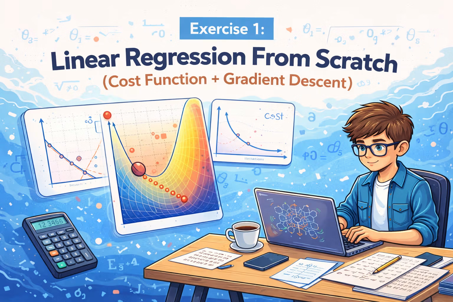
Exercise 1 - Linear Regression From Scratch

Warm-up: “Hello, Octave”

The warm-up is intentionally tiny: return a 5×5 identity matrix.

A = eye(5);

I like this because it confirms the full edit → run → submit loop works before you touch ML logic.

Plot the data (don’t code blind)

If you only do one thing before implementing learning, do this.

In plotData.m, plot x vs y as a scatter plot.

plot(x, y, 'rx', 'MarkerSize', 10);
ylabel('Profit in $10,000s');
xlabel('Population of City in 10,000s');

What I’m looking for:

• does it look roughly linear?
• are there obvious outliers?
• are values in the expected ranges?

Exercise 1’s data looks “linear enough” that a straight line is a reasonable first model.

Build the design matrix X (the Octave mindset)

In this course, you learn to think in matrices early.

For single-variable linear regression, you construct X like this:

• first column: all ones (intercept term)
• second column: the feature values x

m = length(y);
X = [ones(m, 1), x];
theta = zeros(2, 1);

From now on, predictions are just:

predictions = X * theta;

No loops. Cleaner code. Fewer bugs.

Implement computeCost.m (the contract)

computeCost returns a single number: how wrong your current parameters are.

In plain terms:

1. predict all outputs with current theta
2. compute the errors (prediction minus actual)
3. square them
4. average them (with the standard scaling used in the course)

A clean vectorized implementation:

function J = computeCost(X, y, theta)
  m = length(y);
  predictions = X * theta;
  errors = predictions - y;
  J = (1/(2*m)) * (errors' * errors);
end

The single most useful sanity check

With theta = [0; 0], the exercise expects the cost to be approximately:

• J ≈ 32.07

If you don’t get close to that, stop and fix computeCost.m first.

Gradient descent depends on computeCost. If the cost is wrong, “learning” will look like random parameter motion.

Implement gradientDescent.m (the learning loop)

Now we update theta iteratively.

The provided script uses:

• alpha = 0.01
• iterations = 1500

In gradientDescent.m, you:

• compute current errors
• update theta (simultaneously)
• store cost into J_history

Vectorized implementation:

function [theta, J_history] = gradientDescent(X, y, theta, alpha, num_iters)
  m = length(y);
  J_history = zeros(num_iters, 1);

  for iter = 1:num_iters
    errors = (X * theta) - y;
    theta = theta - (alpha/m) * (X' * errors);
    J_history(iter) = computeCost(X, y, theta);
  end
end

What “working” looks like

• J_history decreases over time
• the final line fits the trend on the scatter plot
• your predictions for new x values look plausible

Print cost every ~50 iterations while debugging. This is your training telemetry.

Plot the fitted line on top of the data

Once theta is learned, ex1.m plots the learned line over the scatter plot.

This is the first “wow” moment:

• a couple of functions
• some matrix operations
• and suddenly the computer learns a relationship from data

Visualize the cost surface (why gradient descent works here)

The script explores a grid of parameter values and plots:

• a 3D surface of the cost
• a contour plot

The key intuition you should walk away with:

• for this problem, the cost behaves like a smooth bowl
• there’s a clear lowest point (the best theta)
• gradient descent moves downhill toward that point

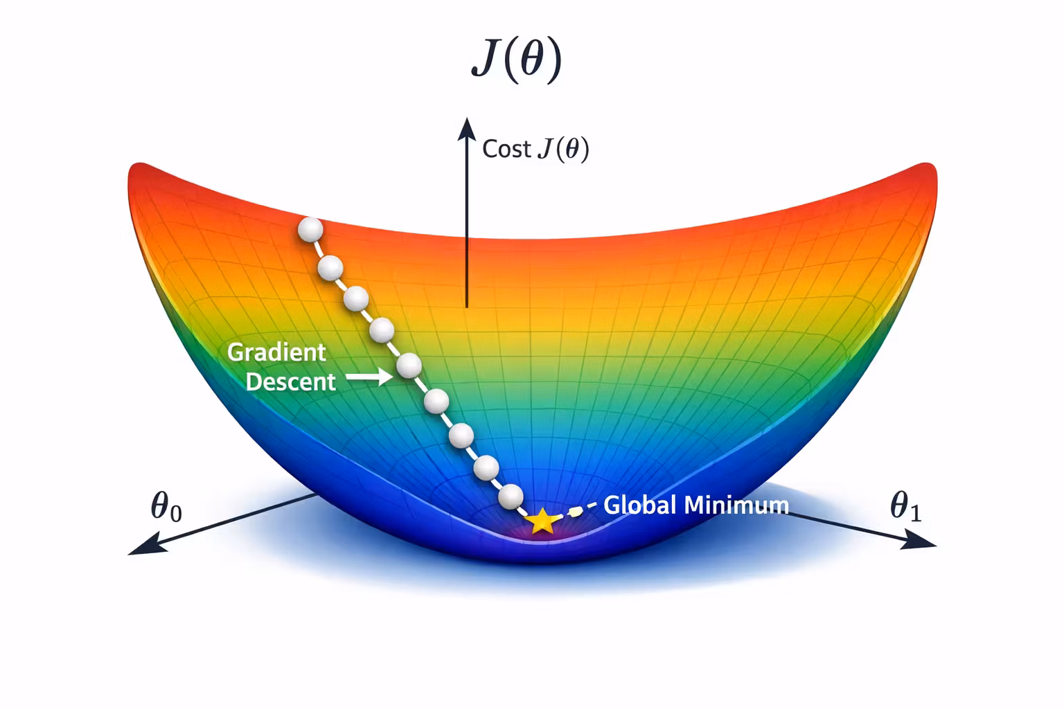
This visualization is why I like Exercise 1: it forces intuition, not just passing tests.