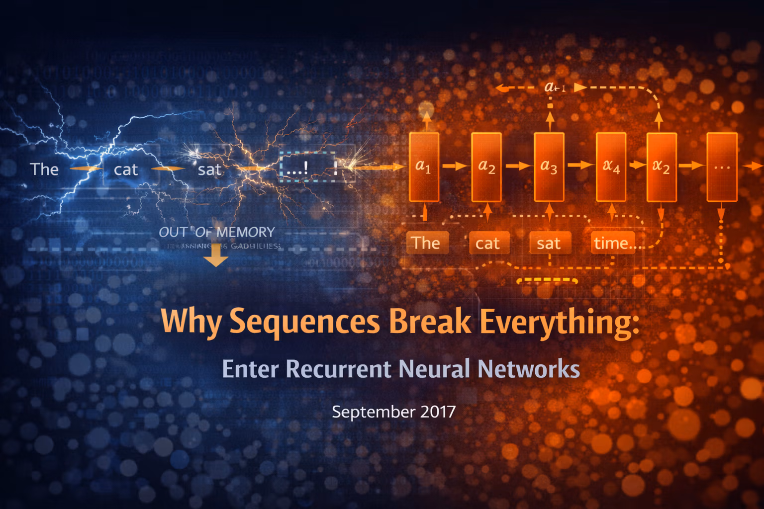
Why Sequences Break Everything - Enter Recurrent Neural Networks

Convolutions taught me something comforting: if you bake the right structure into the model, learning becomes easier.

Then I switched to sequences.

And the comfort disappeared.

Text, sensor streams, audio, click trails… sequences introduce a brutal reality:

order matters, and the past can change the meaning of the present.

In 2016 I could pretend each training example was self-contained.
In September 2017, that illusion broke.

This is the month I met Recurrent Neural Networks — and understood why people say “sequence data breaks everything”.

The Problem That Finally Forced Me Into RNNs

I tried to approach sequence problems with my “classic ML brain”:

• take a window of the last k steps
• engineer features (counts, averages, deltas)
• throw logistic regression / SVM / even a small MLP at it

And it worked… until it didn’t.

The failures were consistent:

• longer context mattered, but my window couldn’t grow forever
• changing k changed the whole problem
• handcrafted features were a guessing game

It felt like vision before CNNs: a messy feature pipeline.

So I asked the obvious question:

Can the model learn the features it needs from raw sequences, the way CNNs learn features from pixels?

That question leads directly to RNNs.

The Core Idea: A Network With Memory (State)

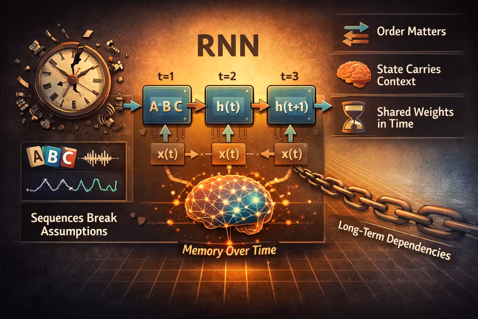
An RNN is just a neural network that keeps a running internal summary:

• at each time step t
• it takes input x(t)
• and the previous hidden state h(t-1)
• and produces a new hidden state h(t)

That hidden state is the “memory”.

Not memory like a database.
Memory like: “what I’ve seen so far.”

This shifted my mental model from:

• “one input → one output”

to:

• “a stream of inputs → evolving internal state → outputs”

Unrolling: The Trick That Made It Click

I kept getting stuck on the word “recurrent” as if it was mystical.

The breakthrough was unrolling.

If you “unroll” an RNN through time, you don’t see a loop anymore.
You see a stack of repeated cells:

• same computation repeated at each time step
• same weights shared across steps
• different inputs each step
• different state each step

Once I saw it unrolled, it stopped being exotic.

It became:

a deep network where depth = time.

That’s also when I got nervous, because I already know what deep networks do to gradients.

(That’s next month.)

Shared Weights Over Time: Why This Isn’t Just “Another MLP”

CNNs use parameter sharing in space.

RNNs use parameter sharing in time.

That parallel helped me a lot.

• CNN: “this edge detector should work anywhere in the image”
• RNN: “this transformation should apply at every time step”

That means:

• fewer parameters than a “different network per time step”
• generalization across sequence positions
• a consistent way to process variable-length inputs

It also means:

• errors at time step 50 still depend on computations from time step 1
• training becomes sensitive to long chains of influence

The good and the painful come from the same source.

What Makes Sequences Different (And Why My 2016 Assumptions Failed)

1) Independence is gone

In 2016, a training example felt like a standalone row in a table.

In sequences, each element is correlated with neighbors by definition.

Treating time steps as independent is like shuffling a sentence’s words and calling it the same sentence.

2) Input and output shapes aren’t fixed anymore

With most classical ML:

• input size is fixed
• output size is fixed

With sequences, you can have different patterns:

• one output for the whole sequence (sentiment)
• one output per time step (tagging)
• output sequence differs from input sequence (translation-style tasks)

Even if I’m not going near translation yet, just realizing these “shapes of problems” mattered was huge.

3) “Past context” is a learnable object

This was the biggest shift:

Instead of feature engineering for context, the RNN carries context forward as state.

Data order is not noise.

Data order is information.

The First Practical RNN I Built (Small, Real, and Humbling)

I kept it deliberately simple:

• character-level sequence prediction (predict the next character)
• tiny vocabulary
• short sequences (at first)
• minimal architecture (one recurrent layer + linear output)

The goal wasn’t state-of-the-art.

The goal was to build a system I could debug.

The humbling part:

• it learned local patterns fast
• it struggled with anything requiring longer memory

Which was the perfect setup for October.

Debugging Notes: The New Failure Modes I Didn’t Have Before

“It learns, but only short-term”

This was the most common behavior.

The model starts producing reasonable local sequences (spaces, punctuation patterns), but loses coherence quickly.

That was my first taste of the long-term dependency problem.

“Training is unstable”

I had runs where loss dropped, then exploded.

That was new.
In classic ML, optimization was frustrating but not chaotic.

Here it could be chaotic.

“State becomes a mystery box”

With CNNs, feature maps gave me something to inspect.

With RNNs, the hidden state is harder to interpret.

So I had to add my own debugging tricks:

• print norms of hidden state over time
• check if state saturates
• check gradients (even roughly)

Why This Mattered to Me (Given My 2016 Background)

Last year I learned:

• optimization is the core
• regularization is a discipline, not a trick
• diagnostics tell you what to do next

RNNs made me apply those principles under harsher conditions.

This was still supervised learning.

Still gradients.

Still cost functions.

But the structure changed the battlefield:

• depth isn’t only layers anymore
• depth is time
• and time can be very long

What Changed in My Thinking (September Takeaway)

Data order is information, not noise.

In 2016 I thought of learning as:

mapping inputs to outputs

In 2017, with sequences, I started thinking of learning as:

building a state that carries context forward

That’s a different mental model.

And it makes it obvious why sequence learning deserved its own class of architectures.

What’s Next

I can now describe RNNs confidently.

But I can also see the storm coming.

If unrolling makes an RNN “deep in time”, then training it means gradients have to travel through a long chain of steps.

Next month is about the pain point everyone warned me about:

Vanishing Gradients Strike Back: why naive RNNs fail on long sequences, and why training can explode or stall.

FAQ