Exercise 6 - Support Vector Machines (When a Different Model Just Wins)

Up to this point in the course, I’ve been living in gradient descent land: pick a cost function, compute gradients, iterate, hope for a different outcome.

Then Support Vector Machines show up… and it feels like switching from a DIY engine rebuild to a tool that just wins.

Not because SVMs are magic (they aren’t), but because:

• they often give a strong decision boundary out of the box
• they handle high-dimensional sparse features really well (hello, email text)
• they force you to think clearly about margin vs misclassification

This exercise is split in two halves:

1. SVM intuition on small 2D datasets (linear boundary + Gaussian kernel)
2. Spam classification using a linear SVM (my first “real” classifier)

What This Exercise Taught Me

The starter SVM implementation included in the assignment is designed for compatibility, not performance. For real-world training, the PDF explicitly recommends using a toolbox such as LIBSVM.

Part 1 — SVMs on Toy Datasets (Where Intuition is Born)

The first script is ex6.m. It walks through 3 datasets:

• ex6data1.mat (linear boundary)
• ex6data2.mat (needs a non-linear boundary)
• ex6data3.mat (non-linear + parameter search)

Dataset 1: Linear Boundary + “That One Outlier”

In ex6data1, there’s an obvious gap between the two classes… except for one positive example sitting in a bad place.

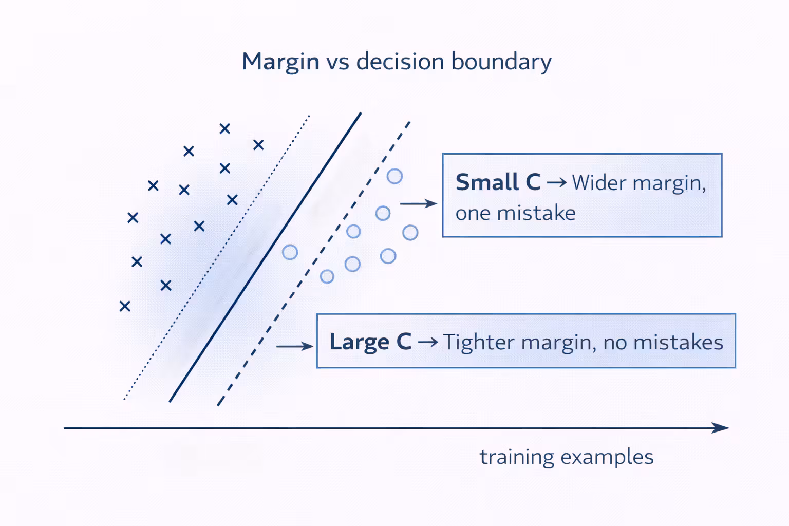
This is the first time the C parameter felt real.

• Small C: prefer a wider margin, tolerate some misclassifications
• Large C: penalize misclassification heavily, try to classify everything correctly

In the assignment we compare:

• C = 1 → boundary stays in the “natural gap” but misclassifies the outlier
• C = 100 → classifies everything correctly, but boundary looks less natural

Engineering interpretation:

• if you crank C up too high, you’re basically saying: “I’d rather contort the boundary than accept a mistake.”
• that’s often a fast route to overfitting.

Implementation detail that bit me once:

Most SVM packages (including the provided svmTrain.m) automatically handle the intercept term. Don’t manually add the x0 = 1 feature like we did for linear/logistic regression.

Part 2 — Gaussian Kernel (Non-Linear Boundaries Without Hand-Crafting Features)

What the Gaussian Kernel is doing

The Gaussian kernel is a similarity function:

• if two points are close → similarity is high
• if they’re far → similarity drops toward zero

A good mental model:

The kernel turns “distance to many landmarks” into new features.

The bandwidth parameter sigma controls how quickly similarity drops:

• small sigma → very local influence (wiggly boundaries)
• large sigma → smoother influence (simpler boundaries)

Implementing gaussianKernel.m

The assignment asks you to implement the kernel and then run a quick test.

The expected value from the provided test case is:

• 0.324652

Here’s a clean Octave-style implementation (no fancy tricks, just vectorization):

function sim = gaussianKernel(x1, x2, sigma)
  x1 = x1(:); x2 = x2(:);
  diff = x1 - x2;
  sim = exp(-(diff' * diff) / (2 * sigma^2));
end

If you can read that code line, you understand the Gaussian kernel: “exponentially down-weight squared distance.”

Dataset 2: Where Linear Just Can’t Cut It

ex6data2 has a layout where no straight line separates the classes well.

Once the Gaussian kernel is used, the learned boundary follows the contours of the dataset and separates most points correctly.

This is the first time in the course I felt a model “bend” the boundary in a controlled way.

Part 3 — Dataset 3: Choosing C and sigma with Cross-Validation

This part is a practical lesson in not guessing hyperparameters.

You’re given:

• training set: X, y
• validation set: Xval, yval

Your job: implement dataset3Params.m to search combinations of C and sigma.

The PDF suggests trying values in multiplicative steps:

• 0.01, 0.03, 0.1, 0.3, 1, 3, 10, 30

That’s 8 values for C and 8 for sigma → 64 models.

The error metric is classification error on the validation set:

pred = svmPredict(model, Xval);
err  = mean(double(pred ~= yval));

Here is the structure I used:

function [C, sigma] = dataset3Params(X, y, Xval, yval)
  values = [0.01 0.03 0.1 0.3 1 3 10 30];
  bestErr = inf;

  for Ctest = values
    for sigTest = values
      model = svmTrain(X, y, Ctest, @(x1, x2) gaussianKernel(x1, x2, sigTest));
      pred  = svmPredict(model, Xval);
      err   = mean(double(pred ~= yval));

      if err < bestErr
        bestErr = err;
        C = Ctest;
        sigma = sigTest;
      end
    end
  end
end

This is the first “real” hyperparameter tuning pattern in the course.

It’s not fancy, but it’s reliable: define a search space, measure on validation, pick the best.

Part 4 — Spam Classification (The Real Payoff)

The second script, ex6spam.m, takes SVMs from toy plots to something useful: spam vs not spam.

This part made SVMs click for me because it combines:

• feature engineering
• preprocessing pipelines
• training + evaluation
• introspection (“what words are the most predictive?”)

Step 1: Email preprocessing (processEmail.m)

The goal: convert raw email text into a list of word indices.

The preprocessing steps are very “classic ML”:

• lower-case everything
• strip HTML tags
• normalize patterns:
  • URLs → httpaddr
  • email addresses → emailaddr
  • numbers → number
  • dollar sign → dollar
• tokenize into words
• apply stemming (Porter stemmer)
• remove punctuation / non-alphanumeric

This is the difference between a model that learns and a model that drowns in noise.

The exercise includes vocab.txt and getVocabList.m which load a fixed dictionary.

This makes the whole pipeline reproducible.

Step 2: Feature extraction (emailFeatures.m)

The dictionary contains 1899 words.

Each email becomes a binary vector x of length 1899:

• x(i) = 1 if vocabulary word i appears in the email
• x(i) = 0 otherwise

After implementing emailFeatures.m, the script checks a sample email and you should see:

• feature vector length: 1899
• number of non-zero entries: 45

That “45” is a nice reminder that these vectors are sparse.

Step 3: Train a linear SVM

The datasets provided are:

• spamTrain.mat → 4000 emails
• spamTest.mat → 1000 emails

Each email is already converted to the 1899-dimensional feature vector using your preprocessing.

The expected performance checkpoint from the assignment:

• training accuracy: ~99.8%
• test accuracy: ~98.5%

That’s absurdly good for such a simple representation.

This is one of the best demonstrations (in the whole course) of why linear models can be incredibly strong when the feature representation is high-dimensional and well-designed.

Top Predictors (What the Model Thinks “Spam” Looks Like)

The script prints the words with the largest positive weights.

From the PDF’s example output, the top predictors include (stemmed forms):

• our
• click
• remov
• guarante
• visit
• basenumb
• dollar
• will
• price
• pleas
• nbsp
• most
• lo
• ga
• dollarnumb

Seeing these terms is a great sanity check: the model is learning patterns that match intuition.

Why This Exercise Matters (Beyond Passing the Autograder)

This was a turning point for me because it’s the first time the course feels like a deployable pipeline:

• preprocess raw input
• map it into features
• train a model
• evaluate on a test set
• inspect what the model learned

And the main engineering lesson:

A “simple” model + strong representation often beats a complex model + messy representation.

My Engineering Notes

What’s Next

Next up, I leave supervised learning behind and step into unsupervised learning.

I’ll implement K-means clustering, compress an image down to 16 colors, then use PCA to reduce dimensions and build intuition for ideas like eigenfaces and variance preservation.