Exercise 5 - Debugging ML (Bias/Variance, Learning Curves, and What to Try Next)

Up to Exercise 4, my workflow was mostly:

• implement the algorithm
• train it
• celebrate when accuracy goes up

Exercise 5 changes the question.

Instead of “can I train a model?”, the question becomes:

My model isn’t performing. What do I try next?

This is the assignment that feels the most like real engineering:

• you train a model
• results look bad
• you diagnose the failure mode
• you apply the right fix (not random tweaks)

The core idea is bias vs variance, and the main tool is learning curves.

What’s inside the Exercise 5 bundle

Why this exercise matters

In production, the painful part of ML is rarely “writing the model.”

The painful part is:

• why is it underperforming?
• am I underfitting or overfitting?
• should I add features, add data, or tune regularization?

Exercise 5 gives you a structured answer.

The dataset (small on purpose)

The first dataset is intentionally tiny.

That’s not a mistake — it’s the point.

A small dataset makes it easier to see:

• what underfitting looks like
• what overfitting looks like
• how adding more data changes the outcome

You start with a simple relationship:

• input: water level
• output: water flowing out

This is “regression,” but the focus is debugging behavior, not the domain.

Step 1 — Regularized linear regression cost + gradient

You implement linearRegCostFunction.m.

It returns:

• J: squared error cost (plus regularization when lambda > 0)
• grad: gradient vector (plus regularization for weights)

Key rule (again):

• do not regularize the bias term (theta(1))

Implementation pattern:

function [J, grad] = linearRegCostFunction(X, y, theta, lambda)
  m = length(y);

  h = X * theta;

  theta_reg = theta;
  theta_reg(1) = 0;

  J = (1/(2*m)) * sum((h - y) .^ 2) + (lambda/(2*m)) * sum(theta_reg .^ 2);

  grad = (1/m) * (X' * (h - y)) + (lambda/m) * theta_reg;
end

If your gradients are wrong, everything after this becomes noise. Validate this function before moving on.

Step 2 — Train with trainLinearReg.m

This helper wraps optimization so the script can repeatedly train models for:

• different training sizes (learning curves)
• different lambda values (validation curve)

The function is simple: it calls an optimizer with your cost function.

This is an important pattern:

• cost + gradients live in one place
• training becomes a reusable “tool”

Step 3 — Learning curves: the best debugging graph in this course

Learning curves plot two errors as you increase the number of training examples m:

• training error
• cross-validation error

The goal is not pretty graphs.

The goal is diagnosis.

How learning curves are computed (important detail)

When building learning curves in this assignment:

• you train using a chosen lambda (often lambda = 0 for the curve)
• but you compute training and validation errors with lambda set to 0

Why?

Because we want to measure pure fit error, not the extra penalty term.

This detail matters or your curves become misleading.

Training uses regularization to prevent crazy parameters. But error reporting uses lambda = 0 so you’re comparing real prediction error.

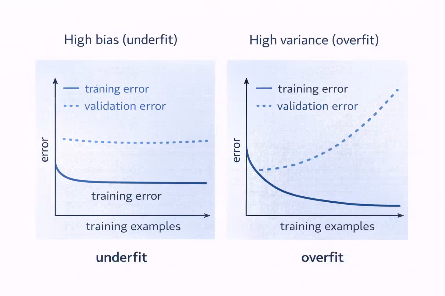
Bias vs variance (the simple decision table)

Step 4 — Polynomial regression (a controlled way to add power)

Next, the assignment has you build polynomial features.

This is a practical move:

• linear regression can underfit if the relationship is curved
• polynomial features make the model more expressive

But as soon as you add polynomial features, you create a new risk:

• overfitting

So the exercise makes you do the full workflow:

• map features
• normalize features
• train
• visualize fit
• diagnose

Feature normalization is not optional here

Polynomial features explode in magnitude:

• x, x^2, x^3, …

Without normalization:

• optimization can become unstable
• parameters become hard to compare
• learning curves become harder to interpret

The provided featureNormalize.m is part of the “real workflow” habit.

Step 5 — Validation curve: choosing lambda like an engineer

Once you have polynomial features, lambda becomes the main knob.

The correct way to pick lambda is:

• choose a set of candidate values
• train a model for each
• evaluate on validation set
• select the lambda with lowest validation error

Typical grid:

lambda in {0, 0.001, 0.003, 0.01, 0.03, 0.1, 0.3, 1, 3, 10}

This assignment formalizes that into validationCurve.m.

Do not use the test set to choose lambda. The test set is the final exam.

The “What to Try Next” playbook (the actual value)

This is the practical output of Exercise 5.

When performance is bad, I now ask:

1) Is this high bias or high variance?

Use learning curves.

2) If high bias, try:

• add more features (polynomial, interactions)
• reduce lambda
• choose a more expressive model

3) If high variance, try:

• increase lambda
• reduce feature mapping
• add more training data

4) If both are bad, try:

• better features (domain-informed)
• check data quality (noise, mislabeled examples)
• confirm splits (training/validation/test)

In real projects, “get more data” isn’t always possible. Regularization and better features are often the first real levers.

Steps I followed (the workflow I want to repeat)

Implement linearRegCostFunction

Validate cost and gradient shapes and ensure bias is not regularized.

Train a baseline linear model

Plot the fit and get an initial sense of underfit/overfit.

Generate learning curves

Compute training and validation error as the training set grows.

Add polynomial features + normalization

Increase model power in a controlled way.

Tune lambda using a validation curve

Select lambda based on validation error, not intuition.

Re-check learning curves with the tuned lambda

Confirm the diagnosis improves (gap shrinks for variance, errors drop for bias).

Debugging checklist (common failure points)

What I’m keeping from Exercise 5

• Learning curves turn “ML debugging” into an actual process.
• Bias vs variance is a decision tool, not a philosophy.
• Lambda is best chosen via validation curves.
• Feature normalization is part of the pipeline, not a bonus.
• “What to try next” is answerable if you measure the right things.

What’s Next

Next up, I build my first spam classifier using Support Vector Machines.

I’ll learn how C and sigma shape decision boundaries, why tuning them feels similar to lambda, and why linear SVMs scale surprisingly well for high-dimensional text data.